Projective Geometry

projective geometry

[prə′jek·tiv jē′äm·ə·trē]

(mathematics)

The study of those properties of geometric objects which are invariant under projection.

McGraw-Hill Dictionary of Scientific & Technical Terms, 6E, Copyright © 2003 by The McGraw-Hill Companies, Inc.

The following article is from The Great Soviet Encyclopedia (1979). It might be outdated or ideologically biased.

Projective Geometry

 

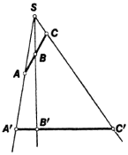
the branch of geometry dealing with the properties of figures that remain invariant under projective transformations—for example, under a central projection. Such properties are called projective properties. The parallelism and perpendicularity of lines and the equality of line segments and angles are not projective properties. For example, the two intersecting lines l and m in Figure 1 are projected to parallel lines l’ and m’, and the two equal segments AB and BC in Figure 2 are projected to the unequal segments A′B′ and B′C′. Since the projection of any conic is a conic, membership in the class of conics is a projective property. Harmonicity of four collinear points, that is, the fact the points form a harmonic set, is also a projective property.

Figure 1

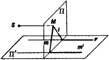
When the points of a plane Π are projected on a second plane Γ as in Figure 1, some of the points of Π lack an image in Π′, and some of the points of Π′ lack a preimage in Π. This makes it necessary to add to the Euclidean plane what are known as ideal points, or points at infinity. As a result, a new geometric entity—the projective plane—is created.

If we add an ideal point to a line, we obtain a projective line. Distinct points are added to nonparallel lines, whereas one and the same point is added to parallel lines. When we supplement the plane with the ideal line, the ideal points of all lines in the plane are assumed to lie on the ideal line. The Euclidean plane supplemented with ideal elements is called the (real) projective plane. In this plane, one and only one line passes through any two distinct points, and any two distinct lines have one and only one common point. When ideal elements are added to the Euclidean plane in order to create the projective plane, projection becomes a one-to-one transformation. Projective space is obtained from Euclidean space in an analogous way.

There are several ways of specifying the real projective plane by means of axioms. The most widespread axiom system is obtained by modifying the system proposed by D. Hilbert as the axiomatic basis of plane Euclidean geometry. The projective

Figure 2

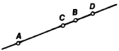
plane is then regarded as a set of two types of elements—points and lines—connected by relations of membership and order, which are described by appropriate axioms. The first group of axioms differs from the corresponding group for Euclidean geometry in that every two lines in the plane have a common point and in that a line has at least three distinct points. The basic order relation is that of separation of two pairs of points on the same line, as described by the second group of axioms. In Figure 3, the pair of points C and D separates the pair A and B, whereas A and C do not separate the pair B and D. These axioms are sometimes supplemented by continuity axioms.

A number of interpretations do not make use of elements at infinity. For example, let R³ be Euclidean space, O a point in R³, and Π the set of lines that pass through O. A Euclidean line passing through O is called a point in Π, and the set of coplanar Euclidean lines passing through O is called a line in Π. The set Π then satisfies the axioms of a projective plane.

Figure 3

Coordinates may be introduced into the projective plane in, for example, the following way. Let IT be the projective plane corresponding to the Euclidean plane Π, and let a Cartesian coordinate system be defined in Π. If M(x, y) is a point in Π, any three numbers (x¹, x², x³) such that x¹/x³ = x and x²/x³ = y are called the homogeneous coordinates of the point M. If ∞ is an ideal point of Π, a pencil of parallel lines passes through it. The homogeneous coordinates of ∞ are any three numbers (x¹, x², x³) such that x¹ and x² are direction numbers of these lines and x³ — 0. Thus, the homogeneous coordinates of a point in Π′ constitute a triple of numbers that do not simultaneously vanish. Any line in the projective plane is determined by the linear homogeneous equation u₁x¹ + u₂x² + u₃x³ = 0 connecting the homogeneous coordinates of the points of this line. Conversely, every such equation determines a line. Number triples (u₁, u₂, u₃) that do not simultaneously equal zero are called homogeneous coordinates of a line. The equation of the ideal line has the form x³ = 0. If the projective plane IT is regarded as a pencil of lines in space, homogeneous coordinates acquire the obvious geometric sense of direction numbers of a line that represents a point in the projective plane. Coordinates in projective space can be introduced in an analogous fashion.

Figure 4

A remarkable feature of projective geometry is the principle of duality. A point and line are said to be incident if the point lies on the line (or the line passes through the point). If some statement A is true of points and lines in the projective plane and is formulated solely in terms of the incidence of these points and lines, the statement B dual to A—that is, the statement obtained from A by replacing the word “point” by the word “line” and the word “line” by the word “point”—is also true.

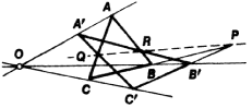
Desargues’s theorem plays an important role in projective geometry. This theorem states that if the corresponding sides of two coplanar triangles ABC and A′B′C′ (Figure 4) intersect at the collinear points P, Q, and R, then the lines joining corresponding vertices are concurrent at the point O. Conversely, if the lines joining corresponding vertices of the coplanar triangles ABC and A ‘B′C′ are concurrent, the corresponding sides of these triangles intersect at collinear points. By the duality principle, the converse of Desargues’s theorem is dual to the direct theorem. Interestingly, this theorem cannot be proved solely on the basis of the incidence axioms of the projective plane. The theorem, however, is true in any projective plane that lies in projective space—for example, the real projective plane. D. Hilbert gave the first example of a projective plane for which Desargues’s theorem does not hold.

Desargues’s theorem is a necessary and sufficient condition for the introduction of coordinates into the projective plane by synthetic means. To do this, we define addition and multiplication of points on the projective line so as to make it into a skew field k. The construction is carried out by using complete quadrangles—that is, plane figures each consisting of four points, no three of which are collinear (Figure 5), and the six lines that join these points in pairs. This configuration makes it possible to define the concept of a harmonic quadruple, or harmonic set, of points in a purely projective fashion. In accordance with duality, the operations of addition and multiplication in a pencil of lines are established by using complete quadrilaterals.

Figure 5

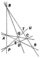
In the synthetic approach to geometry, properties of a projective line as an algebraic system are determined by the geometric properties of the projective plane in which the line is located. We illustrate this fact with two examples. First example: the commutativity of the skew field is equivalent to the fulfillment of Pappus’ theorem, which states that if l and l’ are two distinct lines and A, B, C and A′, B′, C′ are triples of distinct points on l and l’, respectively, then the points of intersection of AB′ and A′B, AC′ and A′C, and BC′ and B′C are collinear. Second example: the skew field k has characteristic not equal to 2 if and only if the diagonal points P, Q, and R of the complete quadrangle ABCD are not collinear; P, Q, and R are defined as the points of intersection of the lines AB and CD, AC and BD, and AD and BC, respectively (Figure 5). In the analytic approach, the properties of a projective line as an algebraic system are determined by the choice of the initial skew field k; different projective planes Π_k can be defined as sets of classes, other than the triple (0,0,0), of proportional triples of elements of different skew fields k. Both approaches can be effectively combined to study the projective properties of curves and surfaces. Analogous constructions can be carried out for projective space.

A conic in the projective plane is defined to within a proportionality factor by a class of homogeneous quadratic equations

a₁₁(x¹)² + a₂₂(x²)² + a₃₃(x³)² + 2a₁₂x¹x² + 2a₂₃x²x³ + 2a₃₁x³x¹ = 0

Every nondegenerate conic, or oval, in the real projective plane is an ellipse, a hyperbola supplemented by the ideal points of its asymptotes, or a parabola supplemented by the ideal point of its diameters. A degenerate conic consists of two distinct or coincident lines or of a single point. Finally, it is possible to have a nondegenerate conic without any real points. This exhausts the projective classification of conics. The figure dual to a conic—or, in this context, a point-conic—is a line-conic, that is, a class of lines determined by a class of proportional homogeneous quadratic equations in the coordinates (u¹, u², u³). A fine-conic can also be described as the set of tangents to a point-conic. The envelope of a line-conic is a point-conic

Figure 6

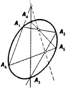
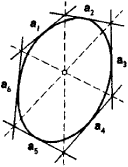
One and only one conic passes through five points in the projective plane when no four of the points are collinear. According to Pascal’s theorem, the points of intersection of the opposite sides of a hexagon inscri bed in a conic are collinear (Figure 6). In the case of a degenerate conic, this theorem reduces to Pappus’ theorem. The dual of Pascal’s theorem is Brianchon’s theorem, which states that the diagonals joining the opposite vertices of a hexagon circumscribed about an oval quadratic curve are concurrent (Figure 7). (See alsoPOLE AND POLAR.)

The foundations of projective geometry were laid in the 17th century by G. Desargues in his development of the science of perspective and by B. Pascal in his study of certain properties of conics. The work of G. Monge in the second half of the 18th century and the early 19th century was of great importance for the subsequent development of projective geometry. Projective geometry was set forth as an independent discipline by J. Poncelet in the early 19th century. Poncelet’s achievement lay in his singling out of the class of projective properties of figures and establishing of correspondences between the metric and projective properties of these figures. The work of the French mathematician C. J. Brianchon also belongs to this period. Projective geometry underwent further development in the work of the Swiss mathematician J. Steiner and the French mathematician M. Chasles. The German mathematician K. von Staudt also played an important role. The outlines of an axiomatic construction of projective geometry are evident in his work. These geometers all attempted to prove theorems in projective geometry by using a synthetic approach based on the projective properties of figures. The outlines of the analytic approach to projective geometry appear in the work of A. Möbius. The development of projective geometry was influenced by N. I. Lobachevskii’s pioneering investigations in non-Euclidean geometry. His investigations permitted A. Cayley and F. Klein subsequently to treat different geometric systems from the standpoint of projective geometry. The development of the

Figure 7

analytic methods of ordinary projective geometry and the construction of complex projective geometry on this basis by the German mathematician E. Study and the French mathematician E. Cartan led to the problem of the dependence of particular projective properties on the skew field over which the geometry is constructed. Important advances toward the solution of this problem have been made by A. N. Kolmogorov and L. S. Pontriagin.

Certain conclusions and findings of projective geometry are made use of in nomography, statistical decision theory, quantum field theory, and the design of printed circuits by means of graph theory.

REFERENCES

Vol’berg, O. A. Osnovnye idei proektivnoi geometrii, 3rd ed. Moscow-Leningrad, 1949.
Glagolev, N. A. Proektivnaia geometriia, 2nd ed. Moscow, 1963.
Efimov, N. V. Vysshaia geometriia, 5th ed. Moscow, 1971.
Hartshorne, R. Osnovy proektivnoi geometrii. Moscow, 1970. (Translated from English.)
Veblen, O., and J. W. Young. Projective Geometry, vols. 1–2. Boston-New York, 1910–18.
Adapted from PROJECTIVE GEOMETRY in the 2nd edition of Bol’shaia Sovetskaia Entsiklopediia.

The Great Soviet Encyclopedia, 3rd Edition (1970-1979). © 2010 The Gale Group, Inc. All rights reserved.